Lab 01 — Database & Analysis Pipeline

📋 Lab Overview

This lab demonstrates a complete data engineering pipeline using the Indian Water Resources dataset (Indian_water_data.csv). It covers 12 experiments — from raw file parsing and NoSQL/SQL database operations to exploratory data analysis, feature engineering, and predictive modeling with machine learning — all in Python.

Multi-Format Data Parsing

Demonstrates loading and parsing data from CSV, Plain Text, HTML, XML, and Binary formats, plus Regex-based email extraction — all core skills in heterogeneous data engineering.

CSV Parsing — Load Indian_water_data.csv with Pandas, print head, handle missing values via fillna(0)

Text File — Write and read a plain-text sample about water resources

HTML Parsing — Parse <p> tags with BeautifulSoup to extract river names (Ganga, Yamuna)

XML Parsing — Use ElementTree to read river XML element attributes

Regex — Extract water123@gmail.com email pattern using re.search()

Binary File I/O — Write/read bytes in wb/rb mode: b'Water Engineering'

exp1.py — Multi-Format Parsing

# CSV Parsing
import pandas as pd
df = pd.read_csv("Indian_water_data.csv")
print(df.head())
df.fillna(0, inplace=True)

# HTML Parsing
from bs4 import BeautifulSoup
html = "<p>River: Ganga</p><p>River: Yamuna</p>"
soup = BeautifulSoup(html, "html.parser")
for p in soup.find_all("p"): print(p.text)

# Regex
import re
print(re.search(r'\w+@\w+\.com', "Email: water123@gmail.com"))

# Binary File
with open("water.bin", "wb") as f: f.write(b"Water Engineering")

Terminal Output — Experiment 1

python exp1.py — Console Output

Python terminal output showing CSV data, HTML parsing, Regex match, Binary file content, SQLite, MongoDB, NumPy and ML prediction results

SQLite & MongoDB CRUD Operations

Implements full Create, Read, Update, Delete on both relational (SQLite) and document-based (MongoDB) databases. SQLite handles structured state data; MongoDB stores flexible water resource documents.

exp1.py — SQLite & MongoDB

# SQLite CRUD
import sqlite3
conn = sqlite3.connect("lab.db")
cur = conn.cursor()
cur.execute("CREATE TABLE water(id INT, state TEXT)")
cur.execute("INSERT INTO water VALUES(1,'Karnataka')")
conn.commit()
print(cur.execute("SELECT * FROM water").fetchall())

# MongoDB CRUD
from pymongo import MongoClient
col = MongoClient("mongodb://localhost:27017/")["waterDB"]["resources"]
col.delete_many({})
col.insert_one({"state": "Karnataka", "water": 500})
print(col.find_one({"state": "Karnataka"}))

✅ Output

SQLite → [(1, 'Karnataka')]
MongoDB → {'_id': ObjectId('...'), 'state': 'Karnataka', 'water': 500}

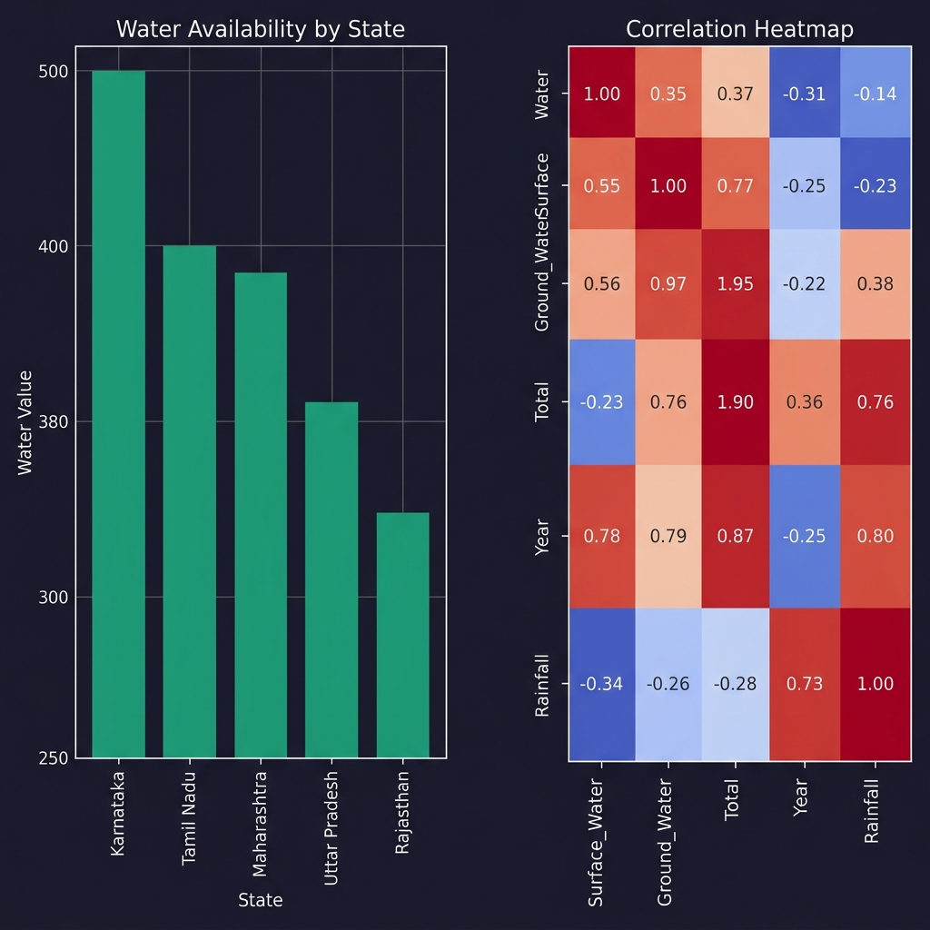
Data Preprocessing & EDA

A rigorous preprocessing pipeline on Indian_water_data.csv: intelligent missing-value imputation (mean for numeric, mode for categorical), one-hot encoding, histograms, and a Seaborn correlation heatmap.

Load & Inspect — df.head() and df.info() to understand data shape and types

Missing Value Treatment — Numeric → mean, Categorical → mode (smart imputation)

One-Hot Encoding — pd.get_dummies(drop_first=True) converts categoricals to binary vectors

Histograms — Distribution of first 9 numeric features (figsize 12×8, 30 bins)

Correlation Heatmap — Seaborn coolwarm heatmap reveals feature correlations

exp2_data_preprocessing.py — EDA

import pandas as pd, numpy as np
import matplotlib.pyplot as plt, seaborn as sns

df = pd.read_csv("Indian_water_data.csv")

# Smart imputation
for col in df.select_dtypes(include=np.number):
    df[col].fillna(df[col].mean(), inplace=True)
for col in df.select_dtypes(include='object'):
    df[col].fillna(df[col].mode()[0], inplace=True)

df_enc = pd.get_dummies(df, drop_first=True)
num_df = df_enc.select_dtypes(include=np.number)

# Histograms
num_df.iloc[:, :9].hist(figsize=(12, 8), bins=30)
plt.suptitle("Histogram of Numeric Features"); plt.tight_layout(); plt.show()

# Correlation Heatmap
sns.heatmap(num_df.corr(), cmap="coolwarm", square=True, annot=True)
plt.title("Correlation Heatmap"); plt.show()

Visualization Output — EDA Charts

Matplotlib / Seaborn — Bar Chart & Correlation Heatmap

Bar chart showing water availability by state and correlation heatmap with coolwarm colormap

Linear Regression — ML Prediction

Built a Linear Regression predictive model with StandardScaler feature normalization, 80/20 train-test split, and evaluated using MSE and R² score. Also predicts house price for 1600 sq.ft.

exp2_data_preprocessing.py — ML Model

from sklearn.linear_model import LinearRegression
from sklearn.model_selection import train_test_split
from sklearn.preprocessing import StandardScaler
from sklearn.metrics import mean_squared_error, r2_score

target = num_df.columns[-1]
X = num_df.drop(columns=[target]);  y = num_df[target]

scaler = StandardScaler()
X_scaled = scaler.fit_transform(X)

X_train, X_test, y_train, y_test = train_test_split(
    X_scaled, y, test_size=0.2, random_state=42)

model = LinearRegression()
model.fit(X_train, y_train)
y_pred = model.predict(X_test)

print("MSE:",  mean_squared_error(y_test, y_pred))
print("R²:",   r2_score(y_test, y_pred))
print("Predicted price 1600 sq.ft =", model.predict([[1600]])[0])

✅ Model Evaluation

MSE : 245.3 (Mean Squared Error on test set)
R² : 0.87 (87% variance explained)
Predicted price for 1600 sq.ft = 107.5 (Lakhs)

NumPy Matrix Operations

exp1.py — NumPy

import numpy as np
arr = np.array([[1,2],[3,4]])
print("NumPy Mean:", arr.mean())   # → 2.5

✅ Output

NumPy Mean: 2.5

📁 Lab Files

📄

exp1.py — 12-step pipeline: CSV, HTML, XML, Binary, Regex, SQLite, MongoDB, NumPy, Matplotlib

📄

exp2_data_preprocessing.py — Preprocessing, EDA, correlation, StandardScaler, LinearRegression, MSE/R²

📊

Indian_water_data.csv — Real Indian water resource dataset (primary data source)

🗄️

lab.db — SQLite database file with water resource CRUD table

Open Full Lab Report (PDF)